
The Cora Dataset
The Cora dataset consists of 2708 scientific publications classified into one of seven classes. The citation network consists of 5429 links. Each publication in the dataset is described by a 0/1-valued word vector indicating the absence/presence of the corresponding word from the dictionary. The dictionary consists of 1433 unique words.

This dataset is the MNIST equivalent in graph learning and we explore it somewhat explicitly here in function of other articles using again and again this dataset as a testbed.
► Direct link to download the Cora dataset
► Alternative link to download the Cora dataset
► GraphML file with applied layout (same as image above)
► The nodes in CSV format
► The edges in CSV format
► Neo4j v5.2 dump to restore (works with v5.9 and below)
►Cora explorations as Jupyter notebook
Download and unzip, say in ~/data/cora/.
    import os
    import networkx as nx
    import pandas as pd
    data_dir = os.path.expanduser("~/data/cora")
Import the edges via pandas:
    edgelist = pd.read_csv(os.path.join(data_dir, "cora.cites"), sep='\t', header=None, names=["target", "source"])
    edgelist["label"] = "cites"
The edgelist is a simple table with the source citing the target. All edges have the same label:
edgelist.sample(frac=1).head(5)
| target | source | label | |
|---|---|---|---|
| 3581 | 72908 | 93923 | cites |
| 5303 | 656231 | 103531 | cites |
| 2005 | 14531 | 592830 | cites |
| 987 | 4330 | 37884 | cites |
| 1695 | 10183 | 1120713 | cites |
Creating a graph from this is easy:
    Gnx = nx.from_pandas_edgelist(edgelist, edge_attr="label")
    nx.set_node_attributes(Gnx, "paper", "label")
A node is hence
    Gnx.nodes[1103985]
{'label': 'paper'}
The data attached to the nodes consists of flags indicating whether a word in a 1433-long dictionary is present or not:
    feature_names = ["w_{}".format(ii) for ii in range(1433)]
    column_names =  feature_names + ["subject"]
    node_data = pd.read_csv(os.path.join(data_dir, "cora.content"), sep='\t', header=None, names=column_names)
Each node has a subject and 1433 other flags corresponding to word occurence:
node_data.head(5)
| w_0 | w_1 | w_2 | w_3 | w_4 | w_5 | w_6 | w_7 | w_8 | w_9 | … | w_1424 | w_1425 | w_1426 | w_1427 | w_1428 | w_1429 | w_1430 | w_1431 | w_1432 | subject | |
|---|---|---|---|---|---|---|---|---|---|---|---|---|---|---|---|---|---|---|---|---|---|
| 31336 | 0 | 0 | 0 | 0 | 0 | 0 | 0 | 0 | 0 | 0 | … | 0 | 0 | 1 | 0 | 0 | 0 | 0 | 0 | 0 | Neural_Networks |
| 1061127 | 0 | 0 | 0 | 0 | 0 | 0 | 0 | 0 | 0 | 0 | … | 0 | 1 | 0 | 0 | 0 | 0 | 0 | 0 | 0 | Rule_Learning |
| 1106406 | 0 | 0 | 0 | 0 | 0 | 0 | 0 | 0 | 0 | 0 | … | 0 | 0 | 0 | 0 | 0 | 0 | 0 | 0 | 0 | Reinforcement_Learning |
| 13195 | 0 | 0 | 0 | 0 | 0 | 0 | 0 | 0 | 0 | 0 | … | 0 | 0 | 0 | 0 | 0 | 0 | 0 | 0 | 0 | Reinforcement_Learning |
| 37879 | 0 | 0 | 0 | 0 | 0 | 0 | 0 | 0 | 0 | 0 | … | 0 | 0 | 0 | 0 | 0 | 0 | 0 | 0 | 0 | Probabilistic_Methods |
5 rows × 1434 columns
The different subjects are:
    set(node_data["subject"])
{'Case_Based',
 'Genetic_Algorithms',
 'Neural_Networks',
 'Probabilistic_Methods',
 'Reinforcement_Learning',
 'Rule_Learning',
 'Theory'}
A typical ML challenges with this dataset in mind:
- label prediction: predict the subject of a paper (node) on the basis of the surrounding node data and the structure of the graph
- edge prediction: given node data, can one predict the papers that should be cited?
You will find on this site plenty of articles which are based on the Cora dataset.
For your information, the visualization above was created via an export of the Cora network to GML (Graph Markup Language), an import into yEd and a balloon layout. It shows some interesting characteristics which can best be analyzed via centrality.
Load into Mathematica
The TSV-formatted datasets linked above are easily loaded into Mathematica and it’s also a lot of fun to apply the black-box machine learning functionality on Cora. As an example, you can find in this gist an edge-prediction model based on node-content and adjacency. The model is poor (accuracy around 70%) but has potential, especially considering how easy it is to experiment within Mathematica.
► Cora in the Wolfram Language
Fetch via PyTorch Geometric
PyTorch Geometric has various graph datasets and it’s straightforward to download Cora:
from torch_geometric.datasets import Planetoid
dataset = Planetoid(root='~/somewhere/Cora', name='Cora')

data = dataset[0]
print(f'Dataset: {dataset}:')
print('======================')
print(f'Number of graphs: {len(dataset)}')
print(f'Number of features: {dataset.num_features}')
print(f'Number of classes: {dataset.num_classes}')

print(f'Number of nodes: {data.num_nodes}')
print(f'Number of edges: {data.num_edges}')
print(f'Average node degree: {data.num_edges / data.num_nodes:.2f}')
print(f'Number of training nodes: {data.train_mask.sum()}')
print(f'Training node label rate: {int(data.train_mask.sum()) / data.num_nodes:.2f}')
print(f'Contains isolated nodes: {data.contains_isolated_nodes()}')
print(f'Contains self-loops: {data.contains_self_loops()}')
print(f'Is undirected: {data.is_undirected()}')
You can also convert the dataset to NetworkX and use the drawing but the resulting picture is not really pretty.
import networkx as nx
from torch_geometric.utils import to_networkx
G = to_networkx(data, to_undirected=True)
nx.draw(G)
PyG has lots of interesting datasets, both from a ML point of view and from a visualization point of view. Below is generic approach to download the data and convert it to NetworkX and GML.
from torch_geometric.datasets import Amazon
import numpy as np
from scipy.sparse import coo_matrix
import networkx as nx
# the name can only be 'Computers' or 'Photo' in this case.
amazon = Amazon(root='~/Amazon', name="Computers");
edges = amazon.data["edge_index"];
row = edges[0].numpy();
column = edges[1].numpy();
data = np.repeat(1, edges.shape[1]);
adj = coo_matrix((data, (row, column)));
graph = nx.from_scipy_sparse_matrix(adj);
nx.write_gexf(graph, "~/graph.gml")
The COO format referred to is a way to store sparse matrices, see the SciPy documentation. As outline below, from here on you can use various tools to visualize the graph.
Loading the dataset in Neo4j using Cypher
Download the two CSV files (nodes and edges) and put them in the import directory of the database (see screenshot). They can't be in any other directory since Neo4j will not access files outside its scope.

Run the queries:
LOAD CSV WITH HEADERS FROM 'file:///nodes.csv' AS row
Create (n:Paper{id:row["nodeId"], subject:row["subject"], features:row["features"]});


LOAD CSV WITH HEADERS FROM 'file:///edges.csv' AS row
Match (u:Paper{id:row["sourceNodeId"]})
Match (v:Paper{id:row["targetNodeId"]})
Create (u)-[:Cites]->(v);
This creates something like 2708 nodes and 10556 edges. You can also directly download this Neo4j v5.2 database dump if you prefer.
Loading the dataset in Neo4j using StellarGraph
Certain packages, like StellarGraph, allow to learn from graphs when stored in a database. This opens up all sorts of possibilities, especially in the context of knowledge graphs, fraud detection and more.
The methods below help to transfer the Cora data to Neo4j as the de facto graph store these days. The technique is really straightforward but do note that the rather large 1433-dimensional vector describing the content of a paper is breaking the Neo4j browser. That is, the network visualizer in Neo4j attempts to load these vectors along with the network structure but this fails even for a single node.
The py2neo package is the way to connect to Neo4j from Python. Simply pip-install this package and connect to the store via something like
graph = py2neo.Graph(host="localhost", port=7687, user="neo4j", password="neo4j")
To start with an empty database you can truncate everything with
empty_db_query = """
MATCH(n) DETACH
DELETE(n)
"""
tx = graph.begin(autocommit=True)
tx.evaluate(empty_db_query)
If you get an error at this point it's likely because of the port or the password.
To load all the nodes use the following:
loading_node_query = """
    UNWIND $node_list as node
    CREATE( e: paper {
        ID: toInteger(node.id),
        subject: node.subject,
        features: node.features
    })
    """
batch_len = 500
for batch_start in range(0, len(node_list), batch_len):
    batch_end = batch_start + batch_len
    # turn node dataframe into a list of records
    records = node_list.iloc[batch_start:batch_end].to_dict("records")
    tx = graph.begin(autocommit=True)
    tx.evaluate(loading_node_query, parameters={"node_list": records})
Similarly, for the edges:
loading_edge_query = """
    UNWIND $edge_list as edge
    MATCH(source: paper {ID: toInteger(edge.source)})
    MATCH(target: paper {ID: toInteger(edge.target)})
    MERGE (source)-[r:cites]->(target)
    """
batch_len = 500
for batch_start in range(0, len(edge_list), batch_len):
    batch_end = batch_start + batch_len
    # turn edge dataframe into a list of records
    records = edge_list.iloc[batch_start:batch_end].to_dict("records")
    tx = graph.begin(autocommit=True)
    tx.evaluate(loading_edge_query, parameters={"edge_list": records})
If you want to use this graph database with StellarGraph, see the docs about stellargraph.connector.neo4j connector.
Visualization
You can easily visualize the dataset with various tools. The easiest way is via the yEd Live by opening this GraphML file. There is also the desktop version of yEd.
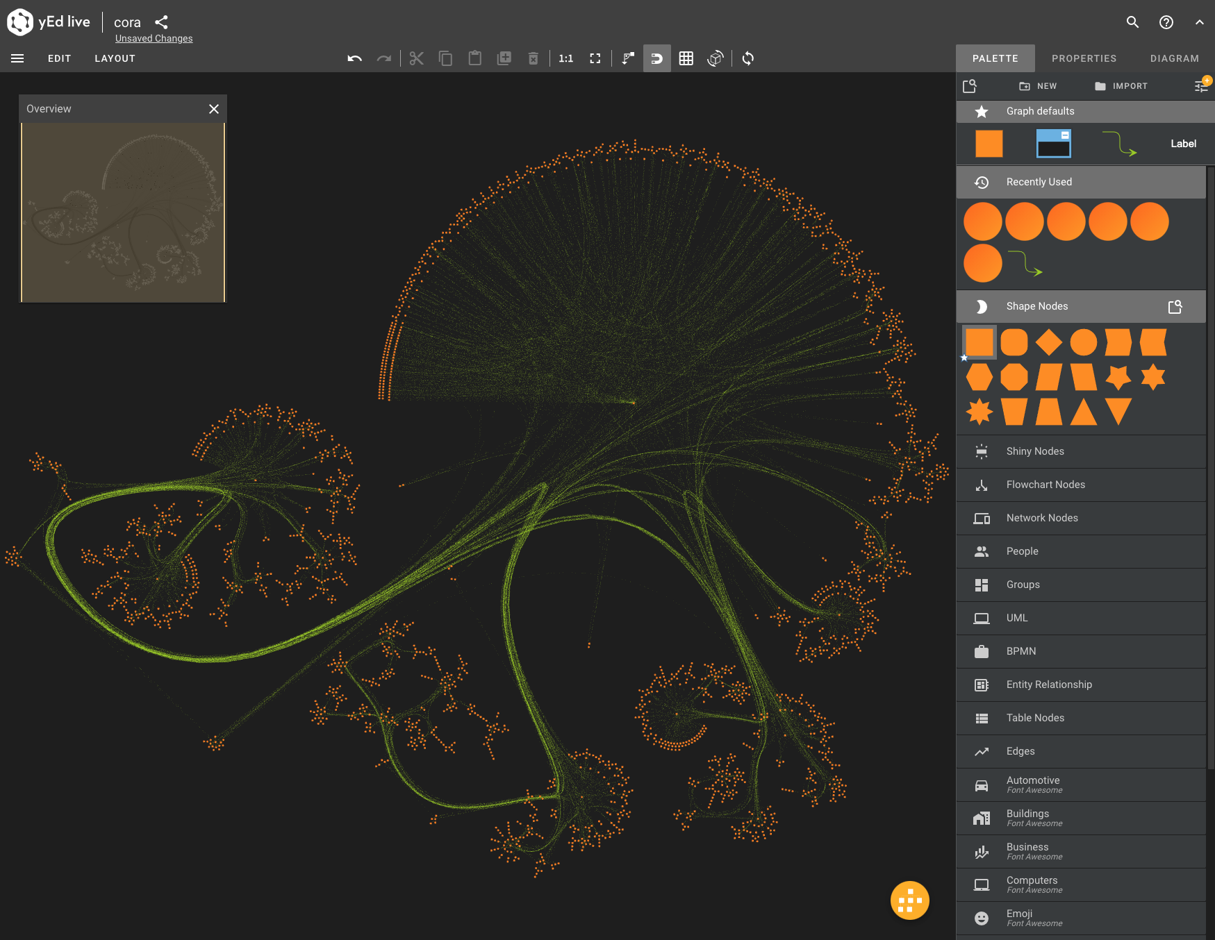
If you wish to reproduce the layout shown, use the balloon layout and use the settings shown below

The Gephi app is a popular (free) app to explore graphs but offers fewer graph layout algorithms. Use this Gephi file or import the aforementioned GraphML file.
Finally, there is Cytoscape and if you download the yFiles layout algorithms for Cytoscape you can create beautiful visualizations with little effort.


